Show the code
pacman::p_load(ggstatsplot, ggthemes, plotly, corrplot, lubridate, ggpubr, plotly, gganimate, viridis, ggridges, ggrepel, testthat, hmisc, tidyverse, funModeling, PMCMRplus, gifski, ggplot2,treemap )In this take-home exercise, we are required to uncover the salient patterns of the resale prices of public housing property by residential towns and estates in Singapore by using appropriate analytical visualisation techniques learned in Lesson 4: Fundamentals of Visual Analytics. Students are encouraged to apply appropriate interactive techniques to enhance user and data discovery experiences.
For the purpose of this study, the focus should be on 3-ROOM, 4-ROOM and 5-ROOM types. You can choose to focus on either one housing type or multiple housing types. The study period should be on 2022.
Resale flat princes based on registration date from Jan-2017 onwards should be used to prepare the analytical visualisation. It is available at Data.gov.sg.
Before we get started, it is important for us to install the necessary R packages into R and launch these R packages into R environment.
The R packages needed for this exercise are as follows:
pacman::p_load(ggstatsplot, ggthemes, plotly, corrplot, lubridate, ggpubr, plotly, gganimate, viridis, ggridges, ggrepel, testthat, hmisc, tidyverse, funModeling, PMCMRplus, gifski, ggplot2,treemap )resale_prices <- read_csv("data/aspatial/resale-flat-prices-based-on-registration-date-from-jan-2017-onwards.csv")summary(resale_prices) month town flat_type block
Length:146872 Length:146872 Length:146872 Length:146872
Class :character Class :character Class :character Class :character
Mode :character Mode :character Mode :character Mode :character
street_name storey_range floor_area_sqm flat_model
Length:146872 Length:146872 Min. : 31.0 Length:146872
Class :character Class :character 1st Qu.: 82.0 Class :character
Mode :character Mode :character Median : 94.0 Mode :character
Mean : 97.6
3rd Qu.:113.0
Max. :249.0
lease_commence_date remaining_lease resale_price
Min. :1966 Length:146872 Min. : 140000
1st Qu.:1985 Class :character 1st Qu.: 358000
Median :1996 Mode :character Median : 448000
Mean :1996 Mean : 478316
3rd Qu.:2007 3rd Qu.: 565800
Max. :2019 Max. :1418000 skimr::skim(resale_prices)| Name | resale_prices |
| Number of rows | 146872 |
| Number of columns | 11 |
| _______________________ | |
| Column type frequency: | |
| character | 8 |
| numeric | 3 |
| ________________________ | |
| Group variables | None |
Variable type: character
| skim_variable | n_missing | complete_rate | min | max | empty | n_unique | whitespace |
|---|---|---|---|---|---|---|---|
| month | 0 | 1 | 7 | 7 | 0 | 74 | 0 |
| town | 0 | 1 | 5 | 15 | 0 | 26 | 0 |
| flat_type | 0 | 1 | 6 | 16 | 0 | 7 | 0 |
| block | 0 | 1 | 1 | 4 | 0 | 2654 | 0 |
| street_name | 0 | 1 | 7 | 20 | 0 | 564 | 0 |
| storey_range | 0 | 1 | 8 | 8 | 0 | 17 | 0 |
| flat_model | 0 | 1 | 4 | 22 | 0 | 21 | 0 |
| remaining_lease | 0 | 1 | 8 | 18 | 0 | 659 | 0 |
Variable type: numeric
| skim_variable | n_missing | complete_rate | mean | sd | p0 | p25 | p50 | p75 | p100 | hist |
|---|---|---|---|---|---|---|---|---|---|---|
| floor_area_sqm | 0 | 1 | 97.60 | 24.09 | 31 | 82 | 94 | 113 | 249 | ▃▇▃▁▁ |
| lease_commence_date | 0 | 1 | 1995.52 | 13.73 | 1966 | 1985 | 1996 | 2007 | 2019 | ▂▇▅▆▇ |
| resale_price | 0 | 1 | 478315.95 | 165533.82 | 140000 | 358000 | 448000 | 565800 | 1418000 | ▆▇▂▁▁ |
town
freq(data=resale_prices,
     input = 'town')
flat_type
freq(data=resale_prices,
     input = 'flat_type')
storey_range
freq(data=resale_prices,
     input = 'storey_range')
floor_area_sqm
freq(data=resale_prices,
     input = 'floor_area_sqm')
lease_commence_date
freq(data=resale_prices,
input = 'lease_commence_date')unique(resale_prices$remaining_lease)resale_price
gghistostats(
  data = resale_prices,
  x = resale_price,
  type = "bayes",
  test.value = 60,
  xlab = "Resale price"
) +
theme_minimal()Separate the years and months.
resale_prices_1 <- resale_prices %>%
  separate(month, c("Year", "Month"), sep = "-")
Convert string to integer.
resale_prices_1$Year <- strtoi(resale_prices_1$Year)
resale_prices_1$Month <- strtoi(resale_prices_1$Month)
convert reaming_lease to reaming_lease_year.
resale_prices_2 <- bind_cols(resale_prices_1,
                              (str_split_fixed(resale_prices_1$remaining_lease,
                                           " ",
                                           4) %>%
                             data.frame() %>%
                             rename(year_lease = X1,
                                    omit1 = X2,
                                    month_lease = X3,
                                    omit2 = X4) %>%
                             select (-c(omit1, omit2)) %>%
                             mutate(month_lease =
                                      ifelse(month_lease == "", 0,
                                             month_lease)) %>%
                             mutate_if(is.character, as.numeric))
                          ) %>%
  mutate (remaining_lease_years = round(year_lease + month_lease/12,2))
derive new variables price_psm,price_thousand,property_age.
resale_prices_3 <- resale_prices_2 %>%
  mutate(price_psm = round(resale_price / floor_area_sqm)) %>%
  mutate(price_thousand = round(resale_price / 1000))
Filter by year 2022
resale_prices_2022 <- resale_prices_3 %>%
filter(Year == "2022", flat_type %in% c("3 ROOM", "4 ROOM", "5 ROOM"))unique(resale_prices_2022$Year)[1] 2022unique(resale_prices_2022$flat_type)[1] "3 ROOM" "4 ROOM" "5 ROOM"summary(resale_prices_2022) Year Month town flat_type
Min. :2022 Min. : 1.000 Length:24372 Length:24372
1st Qu.:2022 1st Qu.: 3.000 Class :character Class :character
Median :2022 Median : 5.000 Mode :character Mode :character
Mean :2022 Mean : 6.047
3rd Qu.:2022 3rd Qu.:10.000
Max. :2022 Max. :12.000
NA's :4450
block street_name storey_range floor_area_sqm
Length:24372 Length:24372 Length:24372 Min. : 51.00
Class :character Class :character Class :character 1st Qu.: 81.00
Mode :character Mode :character Mode :character Median : 93.00
Mean : 94.08
3rd Qu.:110.00
Max. :159.00
flat_model lease_commence_date remaining_lease resale_price
Length:24372 Min. :1967 Length:24372 Min. : 200000
Class :character 1st Qu.:1985 Class :character 1st Qu.: 428000
Mode :character Median :1998 Mode :character Median : 515000
Mean :1997 Mean : 536394
3rd Qu.:2014 3rd Qu.: 610000
Max. :2019 Max. :1418000
year_lease month_lease remaining_lease_years price_psm
Min. :43.00 Min. : 0.000 Min. :43.08 Min. : 3333
1st Qu.:61.00 1st Qu.: 3.000 1st Qu.:61.75 1st Qu.: 4838
Median :74.00 Median : 6.000 Median :74.58 Median : 5368
Mean :74.06 Mean : 5.557 Mean :74.52 Mean : 5736
3rd Qu.:91.00 3rd Qu.: 9.000 3rd Qu.:91.42 3rd Qu.: 6176
Max. :96.00 Max. :11.000 Max. :96.42 Max. :14731
price_thousand
Min. : 200.0
1st Qu.: 428.0
Median : 515.0
Mean : 536.4
3rd Qu.: 610.0
Max. :1418.0
resale_prices_2022_cor <- resale_prices_2022%>%
select (1:2, 8, 10, 15:17)cluster_vars.cor = cor(resale_prices_2022_cor[,3:6])
corrplot.mixed(cluster_vars.cor,
lower = "ellipse",
upper = "number",
tl.pos = "lt",
diag = "l",
tl.col = "black")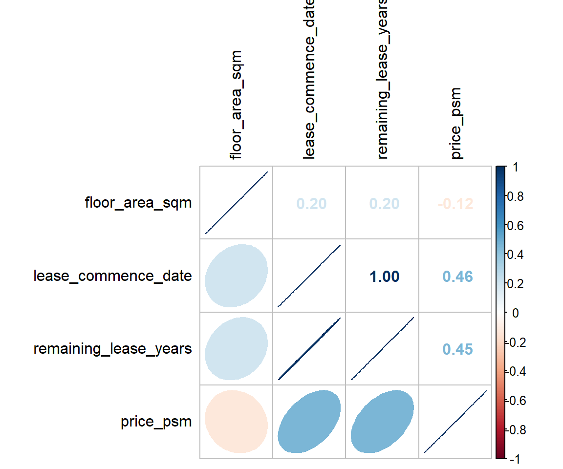
There is no strong correlation amongst the above variables.
set.seed(1234)

resale_prices_2022_3room <- resale_prices_2022 %>%
  filter(flat_type == "3 ROOM")
resale_prices_2022_4room <- resale_prices_2022 %>%
  filter(flat_type == "4 ROOM")
resale_prices_2022_5room <- resale_prices_2022 %>%
  filter(flat_type == "5 ROOM")

p1 <- gghistostats(
  data = resale_prices_2022_3room,
  x = price_thousand,
  type = "bayes",
  test.value = 60,
  xlab = "3 room Price in Thousands") +

  theme_minimal()

p2 <- gghistostats(
  data = resale_prices_2022_4room,
  x = price_thousand,
  type = "bayes",
  test.value = 60,
  xlab = "4 room Price in Thousands") +

  theme_minimal()

p3 <- gghistostats(
  data = resale_prices_2022_5room,
  x = price_thousand,
  type = "bayes",
  test.value = 60,
  xlab = "5 room Price in Thousands") +

  theme_minimal()
ggarrange(p1,p2,p3, ncol = 3, nrow = 1)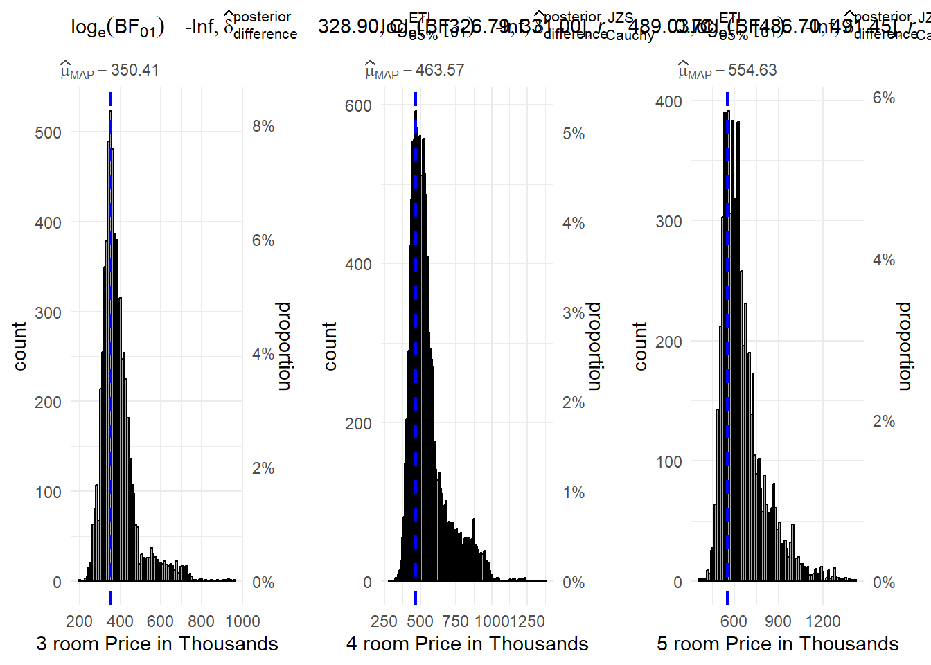
The chart shows, overall, 3 Room price mean is about 350k, 4 Room price mean is about 464K, 5 Room price mean is about 555k.
flat_type_proportion<- resale_prices_2022 %>%
  group_by(town, flat_type) %>%
  summarise(

    n=n())%>%
  mutate(pct_flat = round(n/sum(n)*100))
head(flat_type_proportion)
# A tibble: 6 × 4
# Groups: town [2]
town flat_type n pct_flat
<chr> <chr> <int> <dbl>
1 ANG MO KIO 3 ROOM 528 53
2 ANG MO KIO 4 ROOM 305 31
3 ANG MO KIO 5 ROOM 154 16
4 BEDOK 3 ROOM 555 44
5 BEDOK 4 ROOM 462 36
6 BEDOK 5 ROOM 253 20plot_ly(flat_type_proportion, labels = ~flat_type, values = ~pct_flat, type = 'pie') %>% layout(title = 'Pie chart by flat types in Singapore in 2022',
xaxis = list(showgrid = FALSE, zeroline = FALSE, showticklabels = FALSE),
yaxis = list(showgrid = FALSE, zeroline = FALSE, showticklabels = FALSE))The above chart shows, the top 1 proportion flat type is 4 Room, followed by 3 Room and 5 Room.
flat_type_number<- resale_prices_2022 %>%
  group_by(town, flat_type) %>%
  summarise(

    n=n())

head(flat_type_number)
# A tibble: 6 × 3
# Groups: town [2]
town flat_type n
<chr> <chr> <int>
1 ANG MO KIO 3 ROOM 528
2 ANG MO KIO 4 ROOM 305
3 ANG MO KIO 5 ROOM 154
4 BEDOK 3 ROOM 555
5 BEDOK 4 ROOM 462
6 BEDOK 5 ROOM 253ggplot(flat_type_number,aes(y = reorder(town,n),x = n,fill = flat_type))+
geom_bar(stat = 'identity')+
coord_cartesian(xlim = c(0,3000))+
scale_fill_brewer(palette = "RdBu")+
labs(title = "Number of flats by flat type and by planning area",
x = "Number of flats",
y = "Planning areas in Singapore",
fill = "flat_type")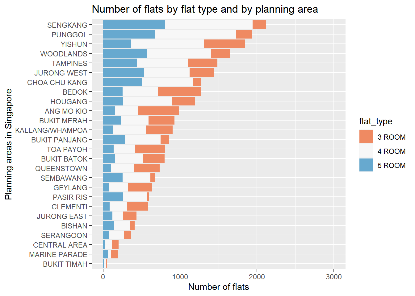
From the above chart, we can see the top 3 areas which have most flats are SENGKANG, PUNGGOL and YISHUN.
ggplot(data = resale_prices_2022, aes(x = price_thousand, y = town, fill = after_stat(x))) +

  geom_density_ridges_gradient(scale = 3, rel_min_height = 0.01) +

  theme_minimal() +

  labs(title = 'Resale Prices by Planning Area in 2022, Month: {frame_time}') +

  theme(legend.position="none",

  plot.title = element_text(face = "bold", size = 12),

  axis.title.x = element_text(size = 10, hjust = 1),
  axis.title.y = element_text(size = 10, angle = 360),
  axis.text = element_text(size = 8)) +

  scale_fill_viridis(name = "price_thousand", option = "D") +

  transition_time(resale_prices_2022$Month) +
  ease_aes('linear')
Visualizing the uncertainty of point estimates
prices_mean_by_town <- resale_prices_2022 %>%
  group_by(town) %>%
  summarise(
    flat_type,
    n=n(),
    mean = round(mean(price_psm)),
    sd=sd(price_psm))%>%

mutate(se=sd/sqrt(n-1))knitr::kable(head(prices_mean_by_town), format = 'html')| town | flat_type | n | mean | sd | se |
|---|---|---|---|---|---|
| ANG MO KIO | 3 ROOM | 987 | 5940 | 1510.833 | 48.11473 |
| ANG MO KIO | 3 ROOM | 987 | 5940 | 1510.833 | 48.11473 |
| ANG MO KIO | 3 ROOM | 987 | 5940 | 1510.833 | 48.11473 |
| ANG MO KIO | 3 ROOM | 987 | 5940 | 1510.833 | 48.11473 |
| ANG MO KIO | 3 ROOM | 987 | 5940 | 1510.833 | 48.11473 |
| ANG MO KIO | 3 ROOM | 987 | 5940 | 1510.833 | 48.11473 |
type <- '3 ROOM'
prices_by_town <- resale_prices_2022 %>% filter(flat_type==type) %>% group_by(town)
ggplot(prices_by_town, aes(x=reorder(town, price_psm), y=price_psm, color = flat_type)) +
  geom_boxplot() +
  labs(title="Flat Resale Price (psm) by Town for 3 Room ",
       x="Town",
       y="Resale Price ($ psm)") +
  theme_classic() +
  theme(plot.title = element_text(size=16, hjust=0.5),
        axis.title.x = element_text(size=15),
        axis.text.x = element_text(angle=45, hjust=1),
axis.title.y = element_text(size=15)) 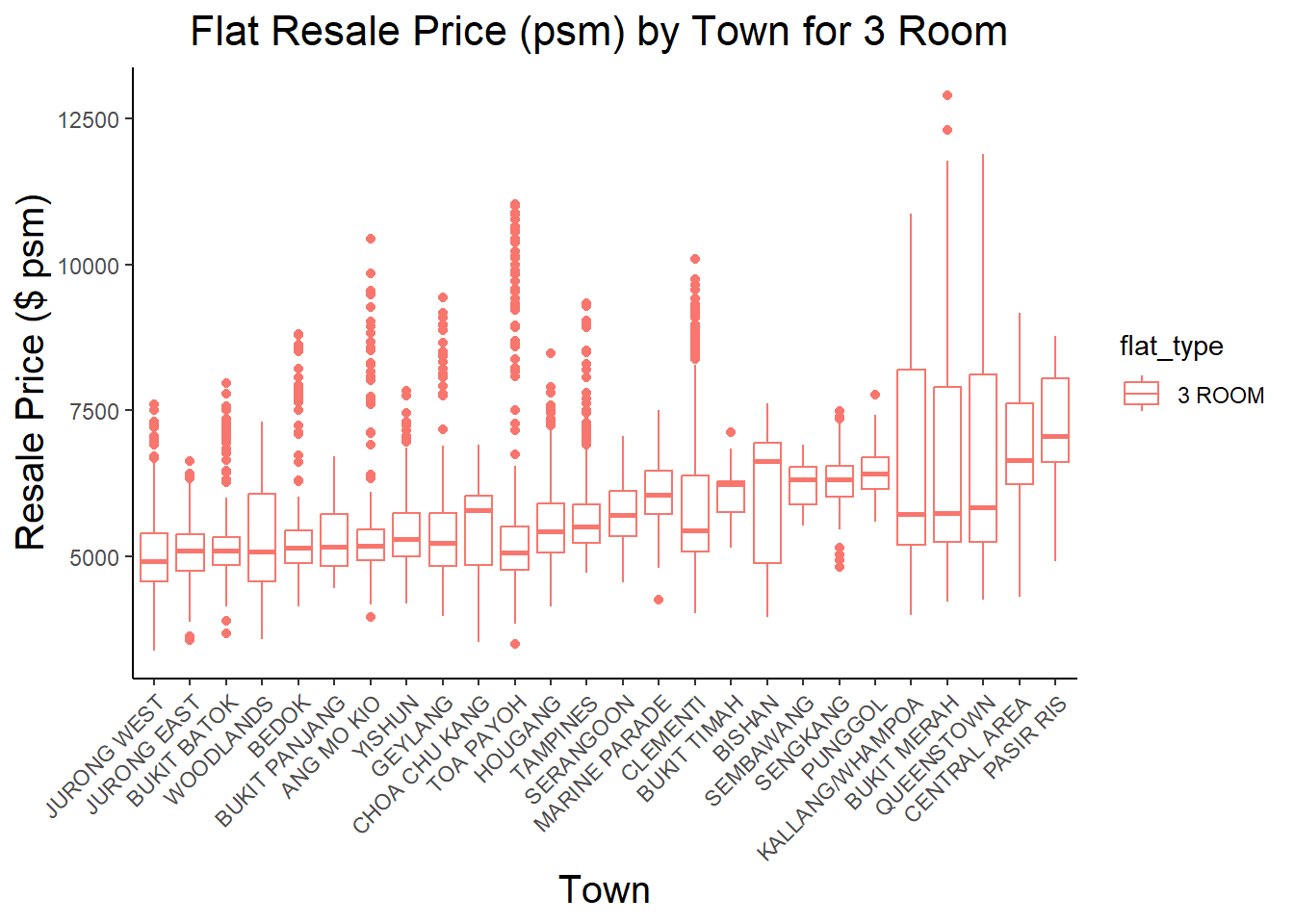
prices_mean_by_town%>%
  filter(flat_type==type)
# A tibble: 6,345 × 6
# Groups: town [26]
town flat_type n mean sd se
<chr> <chr> <int> <dbl> <dbl> <dbl>
1 ANG MO KIO 3 ROOM 987 5940 1511. 48.1
2 ANG MO KIO 3 ROOM 987 5940 1511. 48.1
3 ANG MO KIO 3 ROOM 987 5940 1511. 48.1
4 ANG MO KIO 3 ROOM 987 5940 1511. 48.1
5 ANG MO KIO 3 ROOM 987 5940 1511. 48.1
6 ANG MO KIO 3 ROOM 987 5940 1511. 48.1
7 ANG MO KIO 3 ROOM 987 5940 1511. 48.1
8 ANG MO KIO 3 ROOM 987 5940 1511. 48.1
9 ANG MO KIO 3 ROOM 987 5940 1511. 48.1
10 ANG MO KIO 3 ROOM 987 5940 1511. 48.1
# … with 6,335 more rowsggplot(prices_mean_by_town) +
geom_errorbar(
aes(x=reorder(town,mean),
ymin=mean-se,
ymax=mean+se),
width=0.2,
colour="black",
alpha=0.9,
size=1.5) +
geom_point(aes
(x=town,
y=mean),
stat="identity",
color="red",
size = 1.5,
alpha=1) +
theme_classic() +
theme(plot.title = element_text(size=16, hjust=0.5),
axis.title.x = element_text(size=12),
axis.text.x = element_text(angle=60, hjust=1),
axis.title.y = element_text(size=12)) +
ggtitle("Standard error of 3 Room prices_mean_by_town")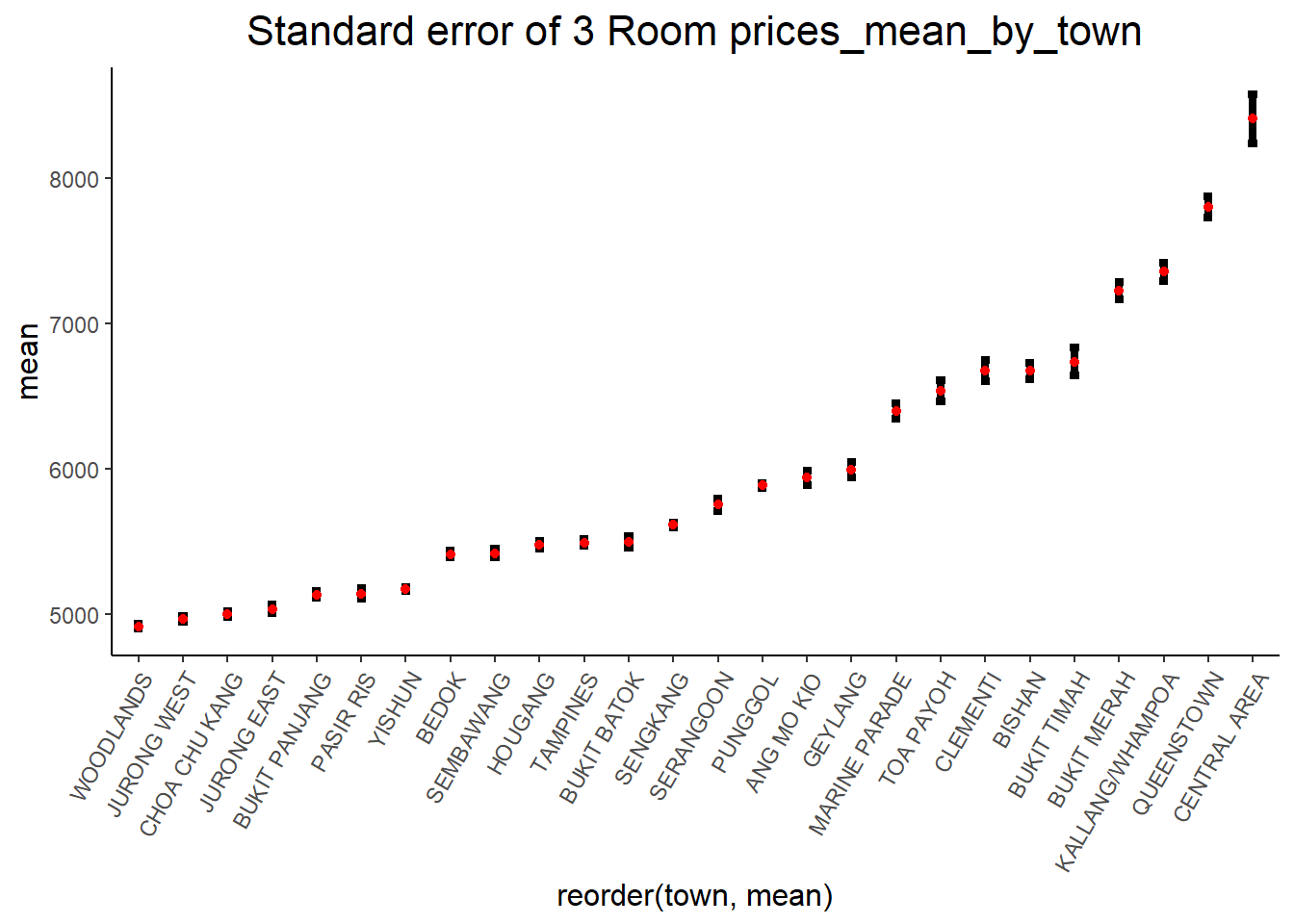
ggarrange(prices_by_town, prices_mean_by_town,ncol = 1, nrow =2 )
The above charts are showing CENTRAL AREA, QUEENSTOWN and KALANG are the top 3 areas which have the higest mean price with 90% of confidence interval.
type <- '4 ROOM'
prices_by_town <- resale_prices_2022 %>% filter(flat_type==type) %>% group_by(town)
ggplot(prices_by_town, aes(x=reorder(town, price_psm), y=price_psm, color = flat_type)) +
  geom_boxplot() +
  labs(title="Flat Resale Price (psm) by Town for 4 Room ",
       x="Town",
       y="Resale Price ($ psm)") +
  theme_classic() +
  theme(plot.title = element_text(size=16, hjust=0.5),
        axis.title.x = element_text(size=15),
        axis.text.x = element_text(angle=45, hjust=1),
axis.title.y = element_text(size=15)) 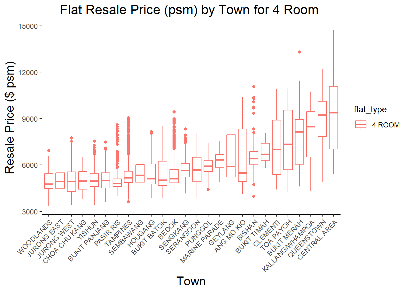
prices_mean_by_town%>%
  filter(flat_type==type)
# A tibble: 11,311 × 6
# Groups: town [26]
town flat_type n mean sd se
<chr> <chr> <int> <dbl> <dbl> <dbl>
1 ANG MO KIO 4 ROOM 987 5940 1511. 48.1
2 ANG MO KIO 4 ROOM 987 5940 1511. 48.1
3 ANG MO KIO 4 ROOM 987 5940 1511. 48.1
4 ANG MO KIO 4 ROOM 987 5940 1511. 48.1
5 ANG MO KIO 4 ROOM 987 5940 1511. 48.1
6 ANG MO KIO 4 ROOM 987 5940 1511. 48.1
7 ANG MO KIO 4 ROOM 987 5940 1511. 48.1
8 ANG MO KIO 4 ROOM 987 5940 1511. 48.1
9 ANG MO KIO 4 ROOM 987 5940 1511. 48.1
10 ANG MO KIO 4 ROOM 987 5940 1511. 48.1
# … with 11,301 more rowsggplot(prices_mean_by_town) +
geom_errorbar(
aes(x=reorder(town,mean),
ymin=mean-se,
ymax=mean+se),
width=0.2,
colour="black",
alpha=0.9,
size=1.5) +
geom_point(aes
(x=town,
y=mean),
stat="identity",
color="red",
size = 1.5,
alpha=1) +
theme_classic() +
theme(plot.title = element_text(size=16, hjust=0.5),
axis.title.x = element_text(size=12),
axis.text.x = element_text(angle=60, hjust=1),
axis.title.y = element_text(size=12)) +
ggtitle("Standard error of 4 Room prices_mean_by_town")
ggarrange(prices_by_town, prices_mean_by_town,ncol = 1, nrow =2 )
The above charts are showing CENTRAL AREA, QUEENSTOWN and KALANG are the top 3 areas which have the higest mean price with 90% of confidence interval.
type <- '5 ROOM'
prices_by_town <- resale_prices_2022 %>% filter(flat_type==type) %>% group_by(town)
ggplot(prices_by_town, aes(x=reorder(town, price_psm), y=price_psm, color = flat_type)) +
  geom_boxplot() +
  labs(title="Flat Resale Price (psm) by Town for 5 Room ",
       x="Town",
       y="Resale Price ($ psm)") +
  theme_classic() +
  theme(plot.title = element_text(size=16, hjust=0.5),
        axis.title.x = element_text(size=15),
        axis.text.x = element_text(angle=45, hjust=1),
axis.title.y = element_text(size=15)) 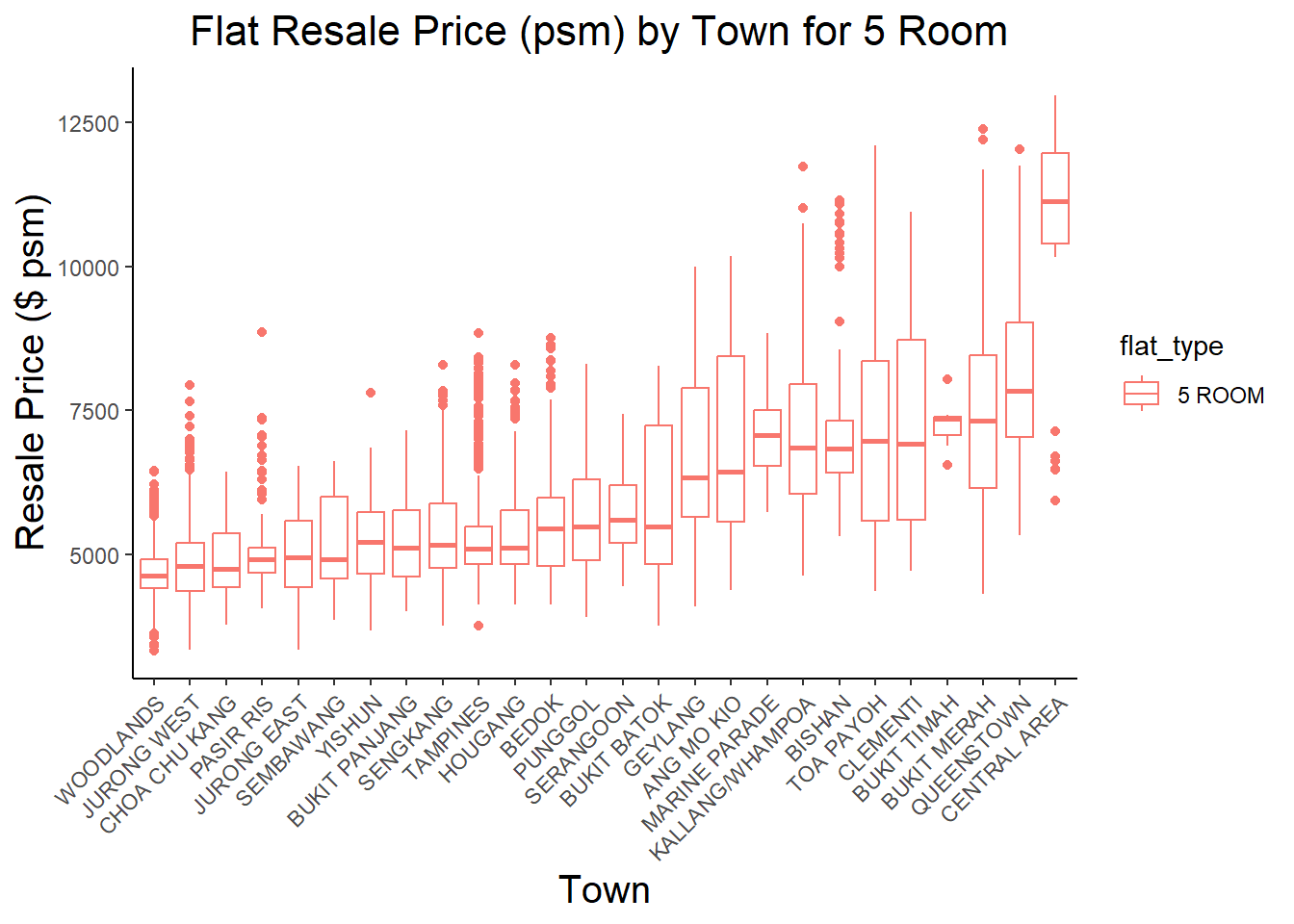
prices_mean_by_town%>%
  filter(flat_type==type)
# A tibble: 6,716 × 6
# Groups: town [26]
town flat_type n mean sd se
<chr> <chr> <int> <dbl> <dbl> <dbl>
1 ANG MO KIO 5 ROOM 987 5940 1511. 48.1
2 ANG MO KIO 5 ROOM 987 5940 1511. 48.1
3 ANG MO KIO 5 ROOM 987 5940 1511. 48.1
4 ANG MO KIO 5 ROOM 987 5940 1511. 48.1
5 ANG MO KIO 5 ROOM 987 5940 1511. 48.1
6 ANG MO KIO 5 ROOM 987 5940 1511. 48.1
7 ANG MO KIO 5 ROOM 987 5940 1511. 48.1
8 ANG MO KIO 5 ROOM 987 5940 1511. 48.1
9 ANG MO KIO 5 ROOM 987 5940 1511. 48.1
10 ANG MO KIO 5 ROOM 987 5940 1511. 48.1
# … with 6,706 more rowsggplot(prices_mean_by_town) +
geom_errorbar(
aes(x=reorder(town,mean),
ymin=mean-se,
ymax=mean+se),
width=0.2,
colour="black",
alpha=0.9,
size=1.5) +
geom_point(aes
(x=town,
y=mean),
stat="identity",
color="red",
size = 1.5,
alpha=1) +
theme_classic() +
theme(plot.title = element_text(size=16, hjust=0.5),
axis.title.x = element_text(size=12),
axis.text.x = element_text(angle=60, hjust=1),
axis.title.y = element_text(size=12)) +
ggtitle("Standard error of 5 Room prices_mean_by_town")
ggarrange(prices_by_town, prices_mean_by_town,ncol = 1, nrow =2 )
The above charts are showing CENTRAL AREA, QUEENSTOWN and KALANG are the top 3 areas which have the higest mean price with 90% of confidence interval.
type <- "3 ROOM"
ggscatterstats(
 data = resale_prices_2022 %>% filter(flat_type==type),
x = remaining_lease_years,
y = price_thousand,
marginal = FALSE)+
  theme_minimal() +
  labs(title=paste("Correlation of Resale Price and Remaining_lease_years", lapply(type, tolower), "flats"), x="Remaining_lease_years", y="Resale Price (in thousand)", fill="Resale Price (in thousand)")+
theme(
        plot.title = element_text(hjust = 0.2, size = 15, face = 'bold'),
        plot.margin = margin(20, 20, 20, 20),
        legend.position = "bottom",

        axis.text = element_text(size = 10, face = "bold"),
        axis.title = element_text(size = 12, face = "bold"))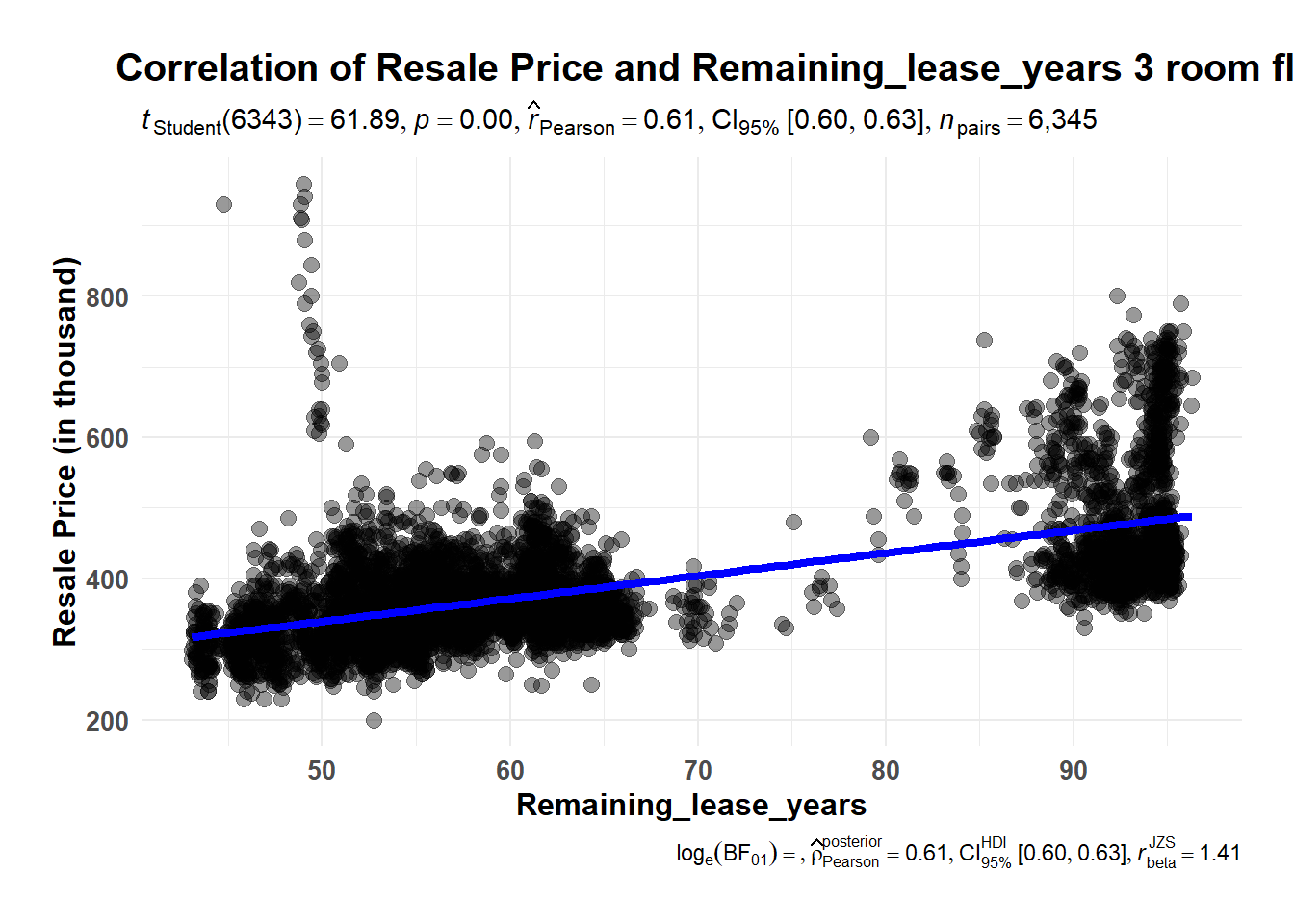
The above chart show the higher remaining lease years, the higher unit price. The coefficient is 0.61 which suggests there is a slight correlation.
type <- '4 ROOM'
ggscatterstats(
 data = resale_prices_2022 %>% filter(flat_type==type),
x = remaining_lease_years,
y = price_thousand,
marginal = FALSE) +
  theme_minimal() +
  labs(title=paste("Correlation of Resale Price and Remaining_lease_years", lapply(type, tolower), "flats"), x="Remaining_lease_years", y="Resale Price (in thousand)", fill="Resale Price (in thousand)")+
theme(
        plot.title = element_text(hjust = 0.2, size = 15, face = 'bold'),
        plot.margin = margin(20, 20, 20, 20),
        legend.position = "bottom",

        axis.text = element_text(size = 10, face = "bold"),
        axis.title = element_text(size = 12, face = "bold"))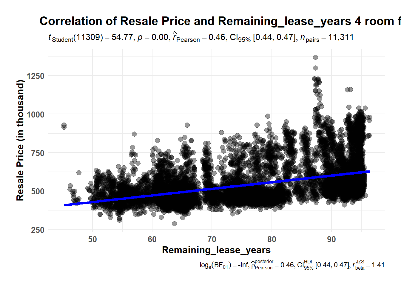
The above chart show the higher remaining lease years, the higher unit price. The coefficient is 0.41 which suggests correlation is not strong.
type <- '5 ROOM'
ggscatterstats(
 data = resale_prices_2022 %>% filter(flat_type==type),
x = remaining_lease_years,
y = price_thousand,
marginal = FALSE) +
  theme_minimal() +
  labs(title=paste("Correlation of Resale Price and Remaining_lease_years", lapply(type, tolower), "flats"), x="Remaining_lease_years", y="Resale Price (in thousand)", fill="Resale Price (in thousand)")+
theme(
        plot.title = element_text(hjust = 0.2, size = 15, face = 'bold'),
        plot.margin = margin(20, 20, 20, 20),
        legend.position = "bottom",

        axis.text = element_text(size = 10, face = "bold"),
        axis.title = element_text(size = 12, face = "bold"))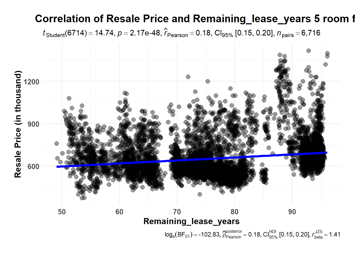
The above chart show the higher remaining lease years, the higher unit price. The coefficient is 0.18 which suggests correlation is not strong.
type <- '3 ROOM'
ggscatterstats(
 data = resale_prices_2022 %>% filter(flat_type==type),
x = floor_area_sqm,
y = price_thousand,
marginal = FALSE) +
  theme_minimal() +
  labs(title=paste("Correlation of Resale Price and floor_area_sqm", lapply(type, tolower), "flats"), x="floor_area_sqm", y="Resale Price (in thousand)", fill="Resale Price (psm)")+
theme(
        plot.title = element_text(hjust = 0.2, size = 15, face = 'bold'),
        plot.margin = margin(20, 20, 20, 20),
        legend.position = "bottom",

        axis.text = element_text(size = 10, face = "bold"),
        axis.title = element_text(size = 12, face = "bold"))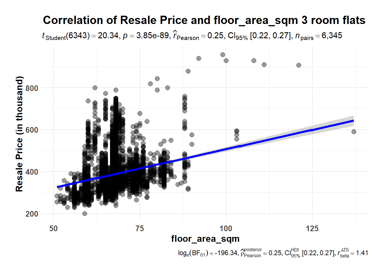
The above chart show the higher remaining lease years, the higher unit price. The coefficient is 0.25 which suggests correlation is not strong.
type <- '4 ROOM'
ggscatterstats(
 data = resale_prices_2022 %>% filter(flat_type==type),
x = floor_area_sqm,
y = price_thousand,
marginal = FALSE) +
  theme_minimal() +
  labs(title=paste("Correlation of Resale Price (psm) and floor_area_sqm", lapply(type, tolower), "flats"), x="floor_area_sqm", y="Resale Price (in thousand)", fill="Resale Price (in thousand)")+
theme(
        plot.title = element_text(hjust = 0.2, size = 15, face = 'bold'),
        plot.margin = margin(20, 20, 20, 20),
        legend.position = "bottom",

        axis.text = element_text(size = 10, face = "bold"),
        axis.title = element_text(size = 12, face = "bold"))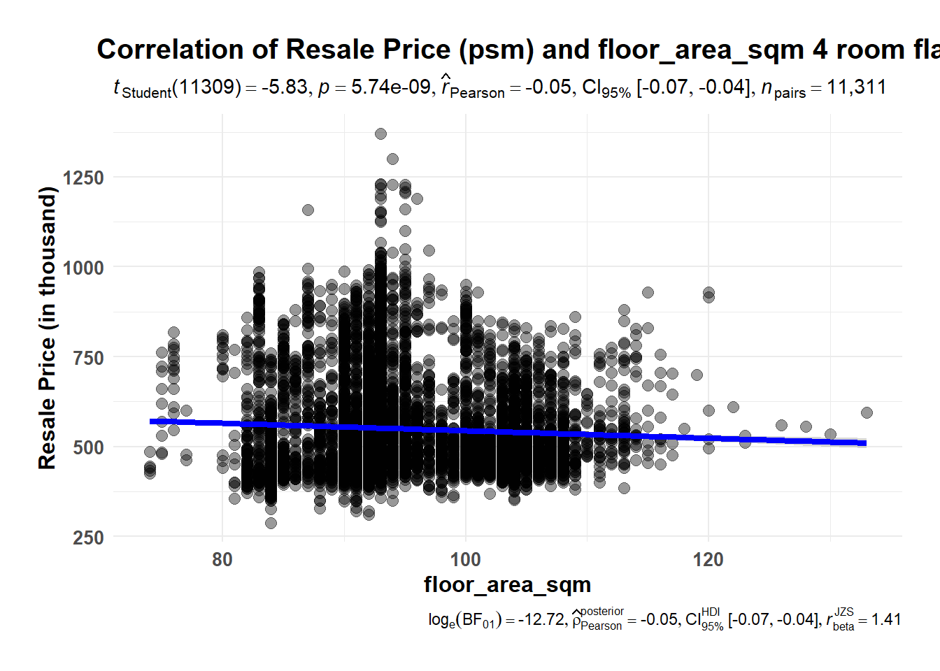
The above chart show the higher remaining lease years, the higher unit price. The coefficient is -0.05 which suggests correlation is not strong.
type <- '5 ROOM'
ggscatterstats(
 data = resale_prices_2022 %>% filter(flat_type==type),
x = floor_area_sqm,
y = price_thousand,
marginal = FALSE) +

  theme_minimal() +

  labs(title=paste("Correlation of Resale Price (psm) and floor_area_sqm", lapply(type, tolower), "flats"), x="floor_area_sqm", y="Resale Price ($ psm)", fill="Resale Price (psm)")+
theme(
        plot.title = element_text(hjust = 0.2, size = 15, face = 'bold'),
        plot.margin = margin(20, 20, 20, 20),
        legend.position = "bottom",

        axis.text = element_text(size = 10, face = "bold"),
        axis.title = element_text(size = 12, face = "bold"))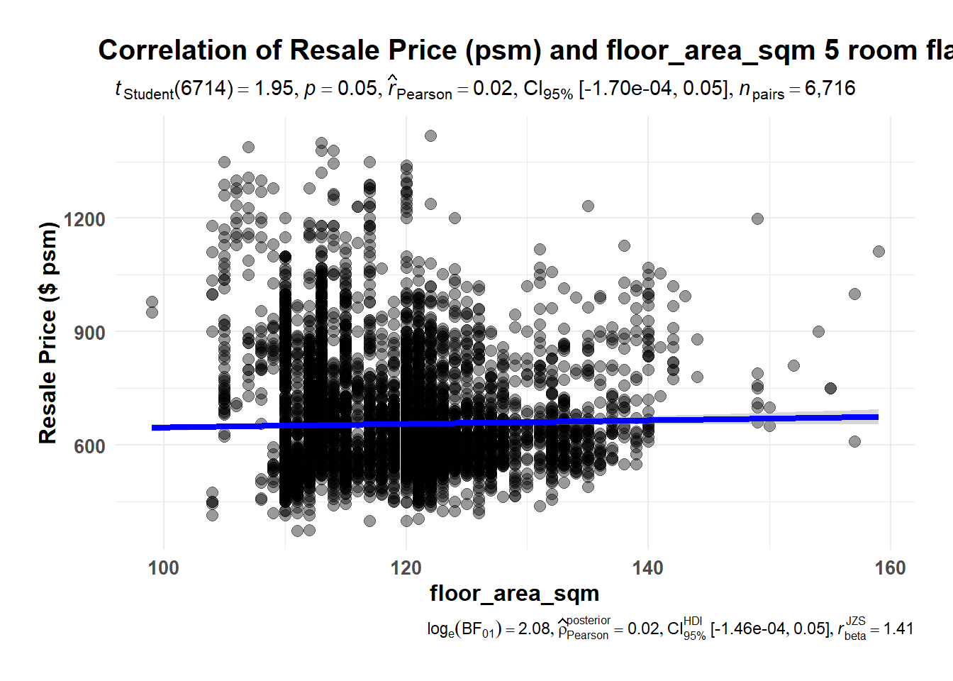
The above chart show the higher remaining lease years, the higher unit price. The coefficient is 0.02 which suggests correlation is not strong.
type <- '3 ROOM'
na.omit(resale_prices_2022) %>%
  filter(flat_type == type) %>%
  ggplot(aes(x = flat_type, y = price_thousand)) +

  geom_boxplot(aes(fill = as.factor(Month)), color = "grey") +

  stat_summary(fun = "mean", geom = "point", color = "black") +

  theme_minimal() +

  scale_fill_brewer(palette = "Paired") +

 labs( title = "Monthly Resale prices by Flat Types",
       y = "Resale price (in thousand)",
       x = "Flat Type",
       fill = "Month") +theme_classic()+

theme(
        plot.title = element_text(hjust = 0.5, size = 12, face = 'bold'),
        plot.margin = margin(20, 20, 20, 20),
        legend.position = "bottom",

        axis.text = element_text(size = 10, face = "bold"),
        axis.title.x = element_text(hjust = 0.5, size = 12, face = "bold"),
        axis.title.y = element_text(hjust = 0.5, size = 12, face = "bold"))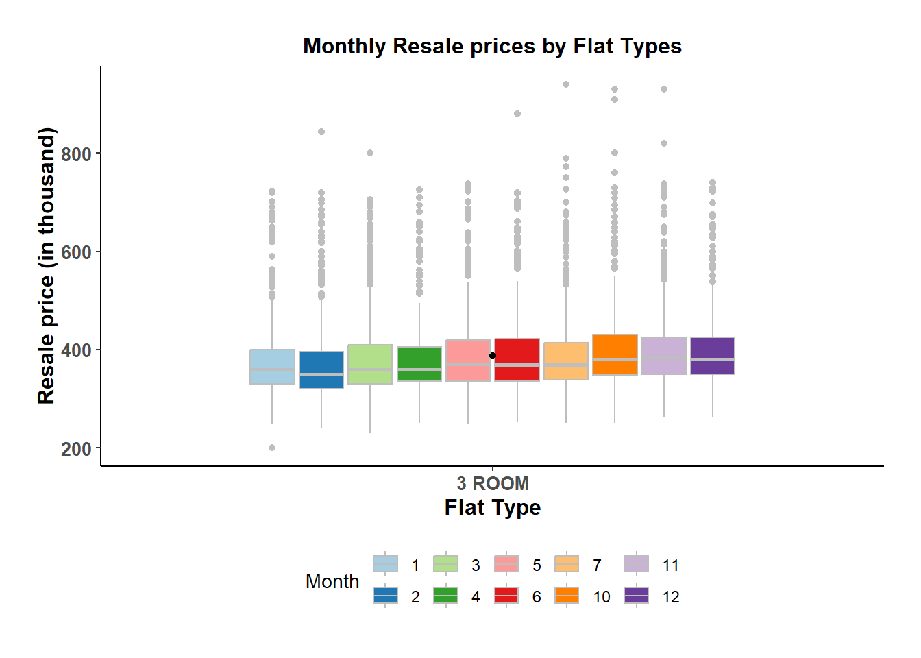
The above chart shows there is no significant increasing or decreasing trend of resale price over months.
type <- '4 ROOM'
na.omit(resale_prices_2022) %>%
  filter(flat_type == type) %>%
  ggplot(aes(x = flat_type, y = price_thousand)) +

  geom_boxplot(aes(fill = as.factor(Month)), color = "grey") +

  stat_summary(fun = "mean", geom = "point", color = "black") +

  theme_minimal() +

  scale_fill_brewer(palette = "Paired") +

 labs( title = "Monthly Resale prices by Flat Types",
       y = "Resale price (in thousand)",
       x = "Flat Type",
       fill = "Month") +theme_classic()+

theme(
        plot.title = element_text(hjust = 0.5, size = 12, face = 'bold'),
        plot.margin = margin(20, 20, 20, 20),
        legend.position = "bottom",

        axis.text = element_text(size = 10, face = "bold"),
        axis.title.x = element_text(hjust = 0.5, size = 12, face = "bold"),
        axis.title.y = element_text(hjust = 0.5, size = 12, face = "bold"))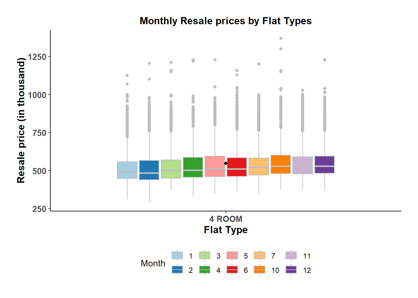
The above chart shows there is no significant increasing or decreasing trend of resale price over months.
type <- '5 ROOM'
na.omit(resale_prices_2022) %>%
  filter(flat_type == type) %>%
  ggplot(aes(x = flat_type, y = price_thousand)) +

  geom_boxplot(aes(fill = as.factor(Month)), color = "grey") +

  stat_summary(fun = "mean", geom = "point", color = "black") +

  theme_minimal() +

  scale_fill_brewer(palette = "Paired") +

 labs( title = "Monthly Resale prices by Flat Types",
       y = "Resale price (in thousand)",
       x = "Flat Type",
       fill = "Month") +theme_classic()+

theme(
        plot.title = element_text(hjust = 0.5, size = 12, face = 'bold'),
        plot.margin = margin(20, 20, 20, 20),
        legend.position = "bottom",

        axis.text = element_text(size = 10, face = "bold"),
        axis.title.x = element_text(hjust = 0.5, size = 12, face = "bold"),
        axis.title.y = element_text(hjust = 0.5, size = 12, face = "bold"))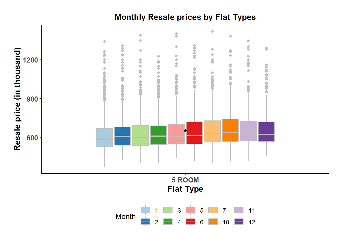
The above chart shows there is no significant increasing or decreasing trend of resale price over months.
#treemap

treemap_storey <- treemap (resale_prices_2022,
        index= c("flat_type", "town"),
        vSize= "price_thousand",
        vColor = "storey_range",
        type="categorical",
        palette = "Blues",
        title="Resale price by storey_range",
        title.legend = "Price_thousand"
        )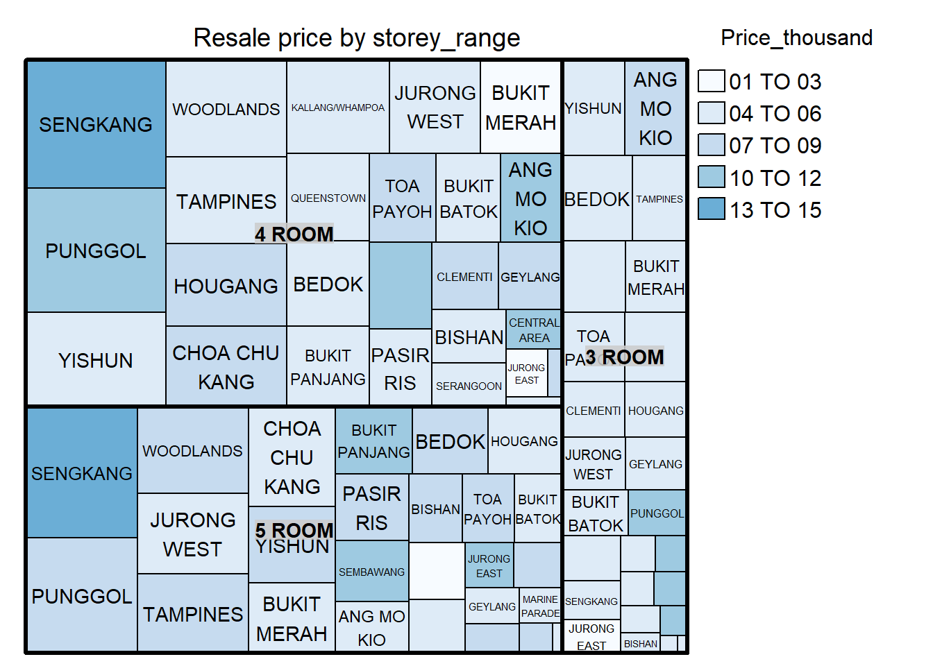
The above chart shows: For 3 Room flat type, the unit prices are higher at YISHUN, ANG MIAO KIAO, BEDOK, storey ranging from 04-06 to 07-09. For 4 Room flat type, the unit prices are higher at SENGKANG, PUNGGOL, YISHUN, storey ranging from 07-09, 10-12 to 13-15. For 5 Room flat type, the unit prices are higher at SENGKANG, PUNGGOL, JURONG WEST, storey ranging from 07-09, 10-12 to 13-15.
Finding 1 - Geography Overall, the top 1 proportion flat type is 4 Room, followed by 3 Room and 5 Room in Singapore in 2022. When looking at the numbers of flats, we can see that SENGKANG, PUNGGOL and YISHUN have the most of the flats of all flat types.This could be seen in section 5.3 Proportion and absolute numbers of flat types in Singapore.
Location had a great effect on flat resale prices. Generally, the CENTRAL AREA had the most expensive flats by mean price per square meter followed by QUEENSTOWN and KALLANG. This could be seen from the box plots and uncertainty of point estimates in section 5.4.2 Average resale prices by room type by planning areas.
Finding 2 - Resale price and remaining lease year, floor area sqm, Time(months) Generally, there is no strong correlation between the unit price and remaining lease, unit price and floor area sqm. This could be seen in section 5.5 Resale price by remaining_lease_year and 5.6 Resale prices by floor_area_sqm.
There is no significant increasing or decreasing trend of resale price over months.This could be seen in section 5.7 resalse price by time(sale months).
Finding 3 - Resale price by storey_range For 3 Room flat type, the unit prices are higher at YISHUN, ANG MIAO KIAO, BEDOK, storey ranging from 04-06 to 07-09. For 4 Room flat type, the unit prices are higher at SENGKANG, PUNGGOL, YISHUN, storey ranging from 07-09, 10-12 to 13-15. For 5 Room flat type, the unit prices are higher at SENGKANG, PUNGGOL, JURONG WEST, storey ranging from 07-09, 10-12 to 13-15. This could be seen in section 5.7 Resale price by storey_range.